Conditional formatting in Excel - what it is and how it works

In large data tables in Excel, it is sometimes necessary to quickly and efficiently identify unusual values, such as values that are too high, too low, that are in a certain range or exceed it, and so on. The most convenient way to do this is through conditional formatting. The conditional formatting changes the appearance of the cells in the table, depending on their content.

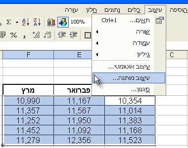
To activate the conditional formatting option, you must mark the desired cell or cells and select the "Conditional Formatting" option in the "Format" menu.

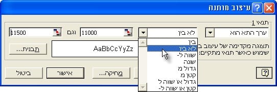
Now the conditions under which the cell design will change must be defined. The first selection field will show "cell value is",
In the second selection field, select the desired option, for example: "not between". In the additional selection fields you must define
the numerical values. In the example in the picture, Excel will change the cell format when the cell value is not between 11,000
and 11,500. In the first selection field you can select "The formula is", and enter a formula that will be used as a condition for the conditional design.
To define several conditions, you can click on the button "Add" >> and define additional conditions according to your choice.

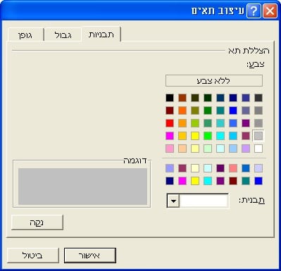
After selecting the conditions, clicking the "Template..." button will open the "Cell design" window. in this window
You can choose how the cells that meet the defined condition will look. In the example in the picture, the cells will be colored gray.

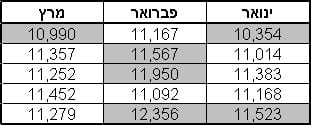
After pressing "OK" in both open windows, the cells that meet the condition will be formatted according to the conditional formatting.
If changes are made to the contents of the cells after the conditional formatting is defined, the formatting will change accordingly.

To apply the conditional formatting to additional cells in the table, or to tables in other sheets, you can simply copy the conditional formatting settings. In order to do so, select one of the designed cells with a right-click and select "Copy".
Now, mark the target cells, and from the "Edit" menu choose "Paste Special". In the window that opens, select "Designs".